EDA, ML and Flask API creation with medical data
Recent advancements in data science render scientists capable of sorting, managing and analyzing large amounts of data more effectively and efficiently. One of the sectors where these new technologies have been applied is the healthcare industry, which is increasingly becoming more data-reliant due to vast quantities of patient and medical data. As a result, medical practices and patient care are significantly improved.
- In this notebook, we will implement various techniques regarding the Exploratory Data Analysis (EDA) of medical data from different datasets and then, train various machine learning models for the prediction of important medical factors. Afterwards, we will export the model that performed the best predictions, we will create a Flask API that performs predictions based on the exported model and finally, we will test the functionality of the created API via Postman.
Exploratory Data Analysis
1st Dataset
The first investigated dataset consists of several thousand measurements of height and weight of males and females. The main information of the imported dataset can be seen below:
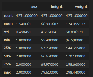
Figure 1: Basic statistics of imported dataset.
We observe that the dataset contains 4231 measurements. We can get more detailed information about the values of each sex:
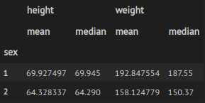
Figure 2: Mean and median height and weight per sex.
By looking at the mean and median values, we can conclude that the values of sex=1 correspond to men’s height and weight.
Data visualisation
A scatter plot is normally fairly informative and very fast to plot.
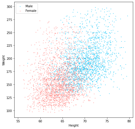
Figure 3: Scatter plot that indicates the sex of each person in each point.
We can see again that most of the women’s weight and height values are mostly smaller than those of men.
We can plot the data based on the sex of each person by taking into account the mean and standard deviation of height and weight.
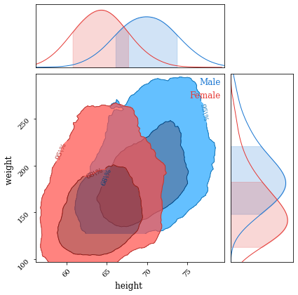
Figure 4: Scatter plot that indicates the sex of each person in each point.
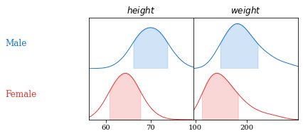
Figure 5: Scatter plot that indicates the sex of each person in each point.
As we can notice in the plots above, mean height and weight of men are greater than those of women.
2nd Dataset
The second dataset of this analysis concerns certain diagnostic measurements originated from the National Institute of Diabetes and Digestive and Kidney Diseases Diabetes dataset. This dataset was obtained from Kaggle. More specifically, all patients here are females at least 21 years old of Pima Indian heritage. The dataset consists of several medical predictor variables and one target variable, Outcome. Predictor variables includes the number of pregnancies the patient has had, their BMI, insulin level, age, and so on.
As a first step, let’s explore the imported dataset.
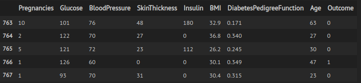
Figure 6: Part of the second dataset.
We observe that there are rows with zero values, thus we can ommit these inputs. After that, we can also get a better summary of the imported data.
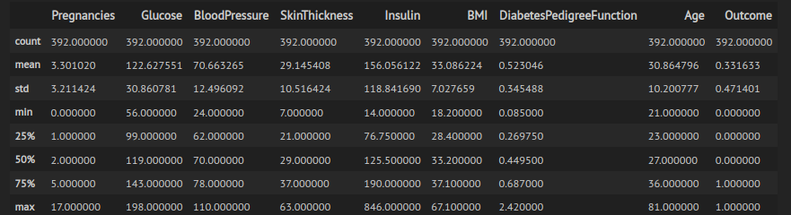
Figure 7: Summary of second Diabetes dataset
Now, the remaining rows are 392.
Data visualisation
We can explore the correlation of the imported data through a heatmap.
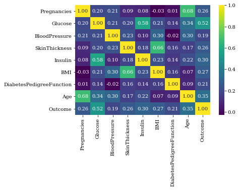
Figure 8: Summary of second Diabetes dataset
In a heatmap like this, the more correlation values are closer to 1 or -1, the more correlated these variables are. For instance, Age and pregnancies are much correlated since the correlation value is 0.68.
Training of machine learning model
Now, let’s keep only three variables that are much correlated with the outcome of the dataset( Diabetes/not Diabetes).
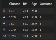
Figure 9: Fraction of dataset used for ML training
We can explore the basic statistics of this dataset.
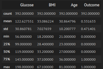
Figure 10: Statistics of dataset used for ML training
Creation of machine learning model in order to predict diabetes cases based on unseen data
By using the above narrowed dataset we trained several models based on various classification algorithms, namely:
- K-Nearest Neighbours
- Support Vector Classifier
- Nu Support Vector Classifier
- Decision Trees
- Random Forest
- AdaBoost
- Gradient Boosting
- Gaussian Naive Bayes
- Linear Discriminant Analysis
- Quadratic Discriminant Analysis
- Multilayer Perceptron.
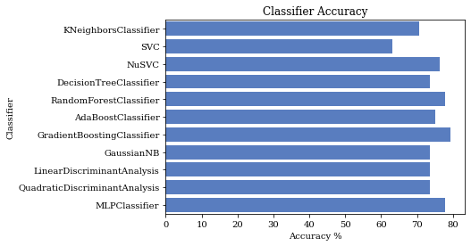
Figure 11: Accuracies of the trained models
According to the calculated accuracies, the best model was K Nearest Neighbour.
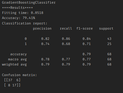
Figure 12: Details of model trained with Gradient Boosting algorithm
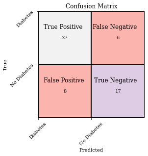
Figure 13: Classification matrix of model trained with Gradient Boosting algorithm
Based on the classifiers’ accuracy, the trained model that performed the best accuracy was Gradient Boosting classifier with accuracy = 79.41%, by showing low log loss : 0.52154. This model, however, showed high Fitting time: Fitting time= 0.0518 sec.
Best model
| Best Model | Accuracy (%) | Log Loss | Fitting Time (s) |
|---|---|---|---|
| Gradient Boosting | 79.41% | 0.52154 | 0.0518 sec |
Creation of Flask API
As a next step, we exported the trained model based on GradientBoosting classifier and created a Flask API. This API takes as input parameters random values of Glucose, BMI and Age, and according to those values, the trained model makes a prediction. A schematic representation of how this API works can be shown below:
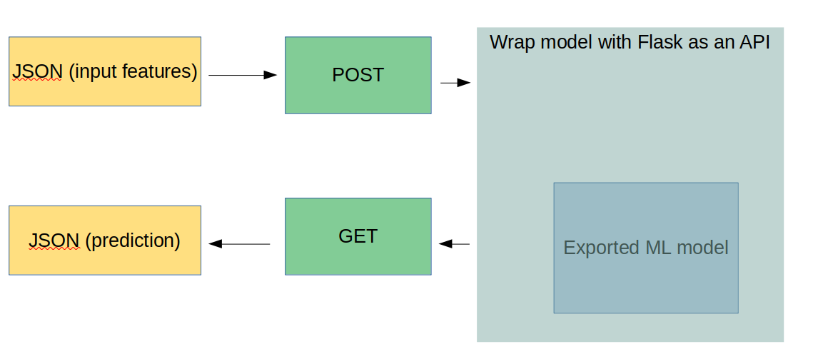
Figure 14: Schematic representation of Flask API's functionality
Afterwards, once we execute the Python that creates the API, we can make several tests through Postman. Some of these tests are illustrated below:
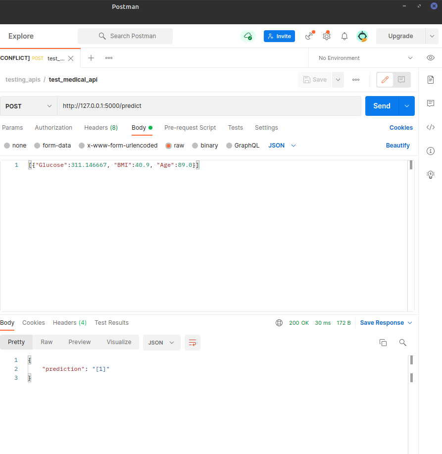
Figure 15: Indicative example of how predictions are made via Flask API
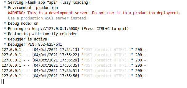
Figure 16: Indicative examples of Flask API requests
A more detailed description of this project’s implementation in Python can be seen in this github repository: Link to Github repository